

pages / notes / 2022 / 2021 / 2020 / 2019 / 2018
Bash commands used to clean the digits copied from the page for the microphone
sensor (remember that the -i switch edits in place and so
over-writes the original file)
sed 's/\(.\)/\1\n/g' -i random.txt # splits so 1 digit per line
sed -i '/^ $/d' random.txt # removes lines with just a space
Then I loaded the random.txt file into RStudio just using the
import data function, which results in a data frame named random. So I pulled
just the digits out of the data frame and plotted a histogram using the
following R commands in the console...
> x <- random[,1]
> hist(x)
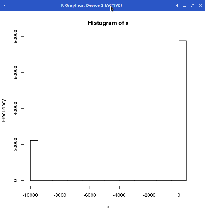
which gave the following plot...

The histogram only has 9 bars - I suspect that the values (0,1] are being
binned as one bar at the beginning (177 zeros and 66 1s and the first
histogram bar is 240 ish high). A barplot from the frequencies
might be better suited to the discrete nature of this data. I used the R
commands below to produce the simple bar chart...
> freqs <- table(x)
> freqs
x
  0   1   2   3   4   5   6   7   8   9
177  66 195  77 146  78 165  63 163  70
> barplot(freqs)

There are way too few odd digits for this data to stand any chance of having a uniform probability distribution! I suspect some kind of rounding or truncating in the analogue to digital conversion that is being used. I'm not sure how the 10 discrete levels recorded are being obtained from the audio output of the microphone.
From the R help function about the chisq.test(vector)
command...
"If x is a matrix with one row or column, or if x is a vector and y is not given, then a goodness-of-fit test is performed (x is treated as a one-dimensional contingency table). The entries of x must be non-negative integers. In this case, the hypothesis tested is whether the population probabilities equal those in p, or are all equal if p is not given."
So the command can be used just from the list of frequencies...
> chisq.test(as.vector(freqs))

	Chi-squared test for given probabilities

data:  as.vector(freqs)
X-squared = 214.18, df = 9, p-value < 2.2e-16

>
And as might be expected, the chi-squared statistic is huge. Re-binning the data into 5 bins (0 and 1, 2 and 3, 4 and 5, 6 and 7, 8 and 9) produces a chi-squared statistic that is much lower and more in line with the assumption of random distribution of outputs...
> rebinned <- c(243, 272, 224, 228, 241)
> chisq.test(rebinned)

	Chi-squared test for given probabilities

data:  rebinned
X-squared = 5.8825, df = 4, p-value = 0.2081

>
The autocorrelation function provides another way of testing for any cyclic disturbance...
> plot(acf(x,plot=F)[1:30])
Resulting autocorrelation plot...

The autocorrelation components are well inside the blue lines that indicate statistical significance so there is no evidence for my original suspicion of a periodic component. Looks like we have a rounding problem.
The page for Sensor Two on the exhibit web site also provides the frequencies for a run of 10000 numbers with a resulting huge chi-square statistic value. Once again, the frequencies for the odd digits are about half those for the even digits, so re-binning to 5 bins produces a dramatic reduction in the statistic...
> y <- c(1271,623,1571,654,1223,671,1430,634,1233,690)
> chisq.test(y)

	Chi-squared test for given probabilities

data:  y
X-squared = 1288.5, df = 9, p-value < 2.2e-16
# rebinned...
> rebiny <- c(1894, 2225, 1894, 2064, 1922)
> chisq.test(rebiny)

	Chi-squared test for given probabilities

data:  rebiny
X-squared = 41.643, df = 4, p-value = 1.978e-08
Take a cooking onion, a couple of cloves of garlic, a can of tomatoes (not the cheapest, plums not chopped) and a good squirt of olive oil or rapeseed oil and a bit of paprika. You can make tomato sauce as follows...
You can add the sauce to freshly cooked pasta, or pop a can of (drained, rinsed) butter beans into the sauce with some dried tarragon as a side dish. Can also be used as a pizza topping base. Customise with basil, salt pepper and so on.
The following spreadsheet formula will simulate rolling a 6 sided dice...
=int(rand()*6 + 1)
And to pick a random digit between 0 and 9 just use...
=int(rand()*9)
This has to do with the Broken Symmetries exhibition at FACT and the work by James Bridle about the difficulties of finding randomness.

The processing sketch below takes about 15 seconds to run on my old i5 laptop. It is almost magic how the dots come up and hug the circle so closely.
/* Monte Carlo PI */
int scale = 500;          /* 1 unit is 500px */
size(600, 600);
float inside = 0;
int MAXGRAINS = 10000000; /* Drop 10 million rice grains */
background(0, 0, 255);
stroke(255,0,0);          /* Each grain is a red dot in a sea of blue */
for(int i = 0; i < MAXGRAINS; i += 1) {
        float x = random(0,1);
        float y = random(0,1);
        float displacement = x*x + y*y;
            if(displacement <= 1.0) {     /* plot if inside */
                  inside = inside + 1.0;     /* count the ones inside */
                  point(scale*x, 600- scale * y);
            }
     }
println(4* inside / MAXGRAINS);  /* print pi estimate to console */

Running the code above generates an estimate of π. Running the simulation 10 times gave the following results...
3.1414776
3.1414060
3.1416273
3.1410017
3.1420412
3.1408553
3.1417055
3.1428697
3.1423693
3.1421740
Dumping these 10 values into R gives...
> summary(x)
   Min. 1st Qu.  Median    Mean 3rd Qu.    Max.
  3.141   3.141   3.142   3.142   3.142   3.143
> boxplot(x)   /* looks symmetrical so trust standard deviation */
> sd(x)
[1] 0.0006507348
> mean(x)
[1] 3.141783
> 2 * sd(x)
[1] 0.00130147

...so we have 4 decimal places of pi by choosing 200,000,000 random numbers and seeing where they fall.

Nassim Nicholas Taleb writes about the implications of rare events with high impact, and about how you manage highly asymmetrical probability distributions. His background is having made enough money in the financial markets to retire from active trading and write his books.
Taleb's early (i.e. pre-2008) book Fooled by Randomness consists of a series of chapters that read like separate articles exploring these themes. In Chapter 6, Skewness and Asymmetry, Taleb proposes a gambling game with two outcomes. Outcome A wins you $1 and has a probability of 0.999. Outcome B costs you $10,000 and has probability 0.001. Taleb then goes on to calculate the expected value of playing this game once (he calls it the 'expectation', I'm using UK maths textbook vocabulary here) as 0.999 × 1 + 0.001 × -10000 = -$9.001. He then comments "Here outcome A is more likely than outcome B. Odds are that we would make money by betting on event A but it is not a good idea to do so".
Taleb suggests that people might fail to distinguish between the probability and expected value because most of their 'schooling' is in 'symmetric environments' such as a coin toss where the expected value mirrors the probability.
I decided to simulate the gambling game so that I could build some
experience in asymmetrical environments. I imagined a large group of
traders (100000) trading for a very long time (100000 days) so that
eventually they would all be cleaned out by the unlikely but serious
outcome B. The result is a kind of life table for traders, because once
cleaned out they cease trading. The c program below comprises a double
loop and a call to the pseudo-random number generator that will provide
an integer between 0 and 999 each with an equal probability of occuring.
The break statement is provided in the inner loop so that
once a trader is cleaned out, they cease to trade. The program prints
the day number at which each trader is cleaned out, one trader to a
line.
/* compile with something like
$ cc taleb.c -lm -o taleb
Nasim's stock market game. Roll a 1000 sided
dice numbered 0 to 999.
If you score 999 you pay $10000.
Else you earn $1.
How many days before you get wiped out?
*/

#include <stdio.h>
#include <stdlib.h>
#include <math.h>
#include <time.h>

#define MAXDAYS 100000 /* can extend to millions in HFT I suppose */
#define MAXTRADERS 100000 /* Lloyds' of London has 34000 names */

int main(void) {
srand(time(0));  /* seed the rng */
int cleaned = 0;
int badnumber = 999;
int droll = 0;
int i, j;
    for(j = 1; j <= MAXTRADERS; j++) {
        cleaned = 0;
        for(i = 1; i <= MAXDAYS; i++) {
            droll = (rand() % 1000);    /* pseudo-random integer between 0 and 999 */
        if (droll == 999) {
            printf("%d \n", i);
            cleaned = 1;
            break;                      /* stop trading if cleaned out */
            }
            } /* end inner loop */
        if (cleaned == 0) {
            printf("S \n");
            } /* end if survived */
    } /* end outer loop */
    printf("\n\n");
    exit(EXIT_SUCCESS);
    } /* end of main */
Running the simulation and redirecting the output to a textfile allows import into R for quick and dirty analysis of the resulting survival data. But first, I check to see if any of the traders has actually survived 100,000 days (very very unlikely unless I made a logic error in the program)...
$ cat taleb.txt | grep  -c S
0
Below are some of the R commands and results. The first thing to do is get my data into R...
> my_data <- read.delim(file.choose()) # choose your file
: taleb.txt
> class(my_data)                     # find out format
[1] "data.frame"
Data frames in R are richer than simple vectors of numbers and they
allow headings, coding of levels and so forth. We don't need any of
those features (yet) so I pull the single column of trader lifetimes in
days into a vector x and eyeball the first few data points
just to check formatting and so on...
> x <- my_data[,1]      # pull a vector out of data frame
> head(x)             # eyeball the first few values
[1] 1148  595  288  721  711  275
Then I use the summary command to calculate the 5-number
summary and mean...
> summary(x)          # basic stats
   Min. 1st Qu.  Median    Mean 3rd Qu.    Max.
    1.0   286.0   688.0   999.3  1378.0 11464.0
The difference between the median and the mean points to a highly skewed distribution and this suspicion is confirmed by the range between the minimum and maximum value. As pointed out by Taleb in a later chapter of the book, that one trader who survived for 11464 days would probably be a media celebrity and have a knighthood by the time (s)he was cleaned out. Noone remembers the ones who lasted less than a couple of years.
A picture lets you see the wood for the trees...
> hist(x) # quick look at distribution
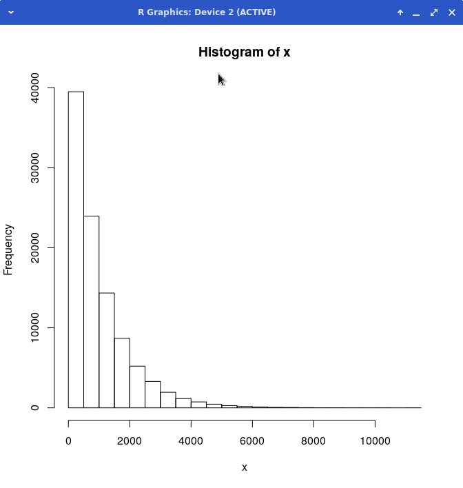
So strongly asymmetrical but looks analytically smooth and 'well behaved'. We can probably model the distribution using one of the classical probability distributions (I'm betting on the poisson).
You can transform highly skewed data so that it looks a little more symmetrical. The logarithm function is a good one for this kind of survival time/nuclear decay like data...
> summary(log10(x))   # transform as very skewed
   Min. 1st Qu.  Median    Mean 3rd Qu.    Max.
  0.000   2.456   2.838   2.750   3.139   4.059
And a picture always helps...
> hist(log10(x)) # visual confirmation, still skewed
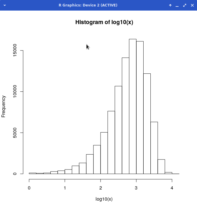
Now the peak is pushed over the other way, so the logarithm function is a tad too agressive a transformation, but the tail is less pronounced.
So much for the probability of surviving as a trader in Taleb's game without being cleaned out. In Chapter 7 of the book, Taleb goes on to look at the outcome for the firm as a whole. He talks about George Soros, Karl Popper and the problem of induction...
"[Soros] knew how to handle randomness, by keeping a critical open mind and changing his opinions with minimal shame (which carries the side effect of making him treat people like napkins)"
The parenthetical comment put me in mind of Soros checking the end of year performance for his (surviving) managers and checking the total profit for the trading firm. The simulation below will generate 250 days worth of data for each of the 100,000 traders. The ones who are cleaned out in the first year are simply escorted from the premises and will show a huge loss for the year. The survivours will have generated $250 each. Lets have a look at the distribution of achieved incomes...
/* compile with something like
$ cc soros.c -lm -o soros
Roll a 1000 sided die (0 to 999).
If you score 999 you lose $10000 and leave to work in
the customer relations side of the fast food industry.
Else you earn $1.
This program calculates the outcome for each trader for a
year's trading.
See Nassim Nicholas Taleb's 'Fooled by Randomness'
Chapter 6 and Chapter 7
*/

#include <stdio.h>
#include <stdlib.h>
#include <math.h>
#include <time.h>

#define MAXDAYS 250         /* Daily deals for one year on LSE */
#define MAXTRADERS 100000   /* Plenty of napkins */
#define OUTCOMEA 1.0        /* Make $1 over the day */
#define OUTCOMEB -10000.0   /* Lose $10000 over the day */

int main(void) {
srand(time(0));  /* seed the rng */
int cleaned = 0;
int badnumber = 999;
int droll = 0;
double total;   /* each trader's annual total */
int i, j;
    for(j = 1; j <= MAXTRADERS; j++) {
        cleaned = 0;
        total = 0.0;
    	for(i = 1; i <= MAXDAYS; i++) {
        	droll = (rand() % 1000);
                if (cleaned == 1) break;  /* trader goes home after loss */
		switch(droll)    {
                      case 999:
                      total = total + OUTCOMEB;
                      cleaned = 1;
                      break;

                      default:
                      total = total + OUTCOMEA;
                      }  /* end of switch...case */
        	} /* end inner loop */
    printf("%f \n", total);  /* one output line per trader */
    } /* end outer loop */
    exit(EXIT_SUCCESS);
    } /* end of main */
Again, running soros and directing the output to
soros.txt will result in a file with the annual results for
100,000 mythical traders. As we know from the survival data above, most
will have survived the first year and made their $250. A smaller
fraction will have been cleaned out. Once again, we use R running in the
same directory as the data file to explore the situation...
> my_data <- read.delim(file.choose())
: soros.txt
> x <- my_data[,1]
> summary(x)
   Min. 1st Qu.  Median    Mean 3rd Qu.    Max.
 -10000     250     250   -2004     250     250
The mean is underwater, on average the firm lost $2000+ per head. However, the vast majority of the traders made their maximum for the year (3rd quartile figure). We have to see what this distribution looks like!
> hist(x)
> sum(x)
[1] -200442872
And there we have why most gamblers and traders would run screaming from this game. It is simply toxic for the firm as a whole. Losing $200 million will not improve the reputation of the firm.
Some tweaking of OUTCOMEA and OUTCOMEB values may result in the firm as a whole breaking even, and then a future continuation of the simulation could put my imaginary George Soros figure in full Popperian control of the company making rational corrections at each stage of a random walk unfolding over a period of years. Unless I can add a few other firms into the market I am unlikely to be able to provoke chaotic behaviour but I will see what I can do.
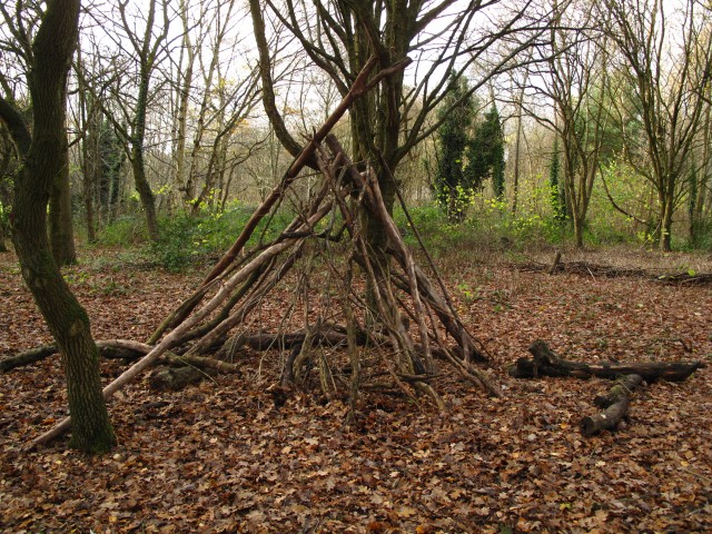
How to program a computer to recognise human structures...Looking for absence of self-similarity?
"...Each of his bread recipes is a variation on a simple formula: 1000 grams flour, 680 grams of water, 20 grams of salt and 20 grams of fresh yeast."
Ken Forkish Flour, water, salt, yeast p42
My basic recipe is: 500g flour and 325g water mixed to rough dough and left for 20 minutes to an hour; mix in 1/8 teaspoon of instant yeast and leave for 5 min; add 1 teaspoon of salt and mix in; knead for 10 minutes; ferment overnight (12 to 16 hours) in mixing bowl covered with a damp teatowel; fold dough and shape into boule; leave to proof for 1 to 2 hours; bake in a cast iron casserole on an oven at maximum temperature (240 to 250 degrees) for 40 minutes and check fully cooked.
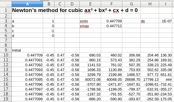
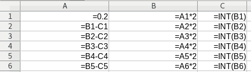
Newton's method for solving an equation by improving on an initial guess is a popular example of a system with fractal basins of attraction to each of the roots of the equation for anything of higher order than a quadratic. I'm fond of this example because it originally surfaced during a teaching session according to Gleick's Chaos. The spreadsheet setup below allows an exploration of the general cubic equation for various starting values and up to 30 iterations. The starting values are shown in the A column and successive iterations are in columns B, C and so on to AD or so. The top of the spreadsheet is used to store the coefficients of the cubic and the range of the starting guesses.
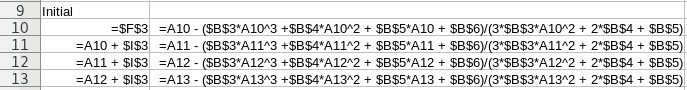
The formulas below show the iteration term and the use of absolute references to include the coefficients and the increment in the starting value for each row.
As you can see, the initial guess x = 0.4477095 results in a spectacular divergence initially, resulting in the solution +1 after 34 iterations. The next larger initial guess at x = 0.4477096 converges on the -1 solution. The basin boundary is between those two initial guesses. The group of positive x values above 0.4477096 are attracted to the -1 solution for a few tenths of x, then the +1 solution arrives again.
The full story awaits an exploration of starting guesses ranging over the complex plane, and that will mean graphics with a square array of initial guesses.


An occasional and subjective review...
/* Random dots to canvas */
size(640, 480);
background(255);
String fn = "";
for(int i = 0; i < 1000001; i += 1) {
        point(random(1,640),random(1,640));
        if((i % 1000) == 0) {
             fn = str(i) + ".png";
             save(fn);
        }
    }
Looks like processing is the environment to use for messing about with fractals. Bottom up programming, built in image save routines, and a handy little movie making tool built in. Above is a minimal framework for plotting dots and saving a frame every thousand iterations or so.
"It seems to me, as just a layman and an amateur, that the internet is almost the perfect distillation of the American capitalist ethos, a flood of seductive choices. It's completely laissez-faire, with no really effective engines for choosing or searching and everybody being much more interested in the economic and material aspects of it than some of the aesthetic and ethical and moral and political questions attached to it."
David Foster Wallace
The iterated sawtooth map is a relatively well-analysed chaos generator.
Compiling and running this...
/* compile with something like
$ cc smale.c -lm -o smale
Iterated mapping is also known as sawtooth map,
bernouilli map &c see page 66 of Gleick's Chaos
*/

#include <stdio.h>
#include <stdlib.h>
#include <math.h>

#define MAXITS 100 /* can extend to millions */

int main(void) {
int numerator = 2;
int denominator = 5;
int i;
    for(i = 1; i <= MAXITS; i++) {
        printf("%d/%d\t", numerator, denominator);
	/* put a newline every 10th result */
        if(i % 10 == 0) printf("\n");
	numerator = numerator * 2;
        if(numerator >= denominator) {
            numerator = numerator - denominator;
            }
        }
    exit(EXIT_SUCCESS);
    }
...results in this 4-cycle as expected...
bash-4.2$ ./smale
2/5	4/5	3/5	1/5	2/5	4/5	3/5	1/5	2/5	4/5
3/5	1/5	2/5	4/5	3/5	1/5	2/5	4/5	3/5	1/5
2/5	4/5	3/5	1/5	2/5	4/5	3/5	1/5	2/5	4/5
3/5	1/5	2/5	4/5	3/5	1/5	2/5	4/5	3/5	1/5
2/5	4/5	3/5	1/5	2/5	4/5	3/5	1/5	2/5	4/5
3/5	1/5	2/5	4/5	3/5	1/5	2/5	4/5	3/5	1/5
2/5	4/5	3/5	1/5	2/5	4/5	3/5	1/5	2/5	4/5
3/5	1/5	2/5	4/5	3/5	1/5	2/5	4/5	3/5	1/5
2/5	4/5	3/5	1/5	2/5	4/5	3/5	1/5	2/5	4/5
3/5	1/5	2/5	4/5	3/5	1/5	2/5	4/5	3/5	1/5
However, the story on LibreOffice is different as you might expect using a floating point approximation to the fractional quantities. The formulas below...
...give these results in later iterations...

A surprise was that using fractions in LibreOffice also suffers from rounding error suggesting that the fractions are not integer based but are reverse engineered from the floating point representation. Screengrabs below show formulas and results for later iterations...


Row 50 shows double 4/5 as 15/8 somehow, the change in demoninator is very mysterious and suggests rounding error. Row 51 in the version using decimal fractions shows 1.625000... and so that would reverse engineer to 15/8. The rounding error growth shows sensitive dependence on initial conditions. I'll be checking MS Excel next...
The texlive packages in RHEL clones such as CentOS, Scientific Linux or Springdale Linux are old and you only get a small selection. It is better to install from the texlive DVD using the install-tl script, I just install the whole lot using about 5Gb of hard drive space. Once the install completes, you can add the path to the texlive binaries to your .bashrc
However if you then install R using yum, the RHEL texlive packages will be installed over your texlive 2018 installation and things won't work. Those clever people at CTAN have a solution: install a dummy texlive package that makes yum think you have the RHEL/CentOS/Springdale/Scientific Linux texlive packages installed, then install texlive 2018 from the DVD and then install R and download and install RStudio.
Commands on this system today...
# yum install R
# yum install perl-Digest-MD5
# rpm -Uvh texlive-dummy-2012a-1.el7.noarch.rpm
# cd /run/media/keith/TeXLive2018 # previously burned to DVD
# ./install-tl
# rpm -Uvh rstudio-1.1.463-x86_64.rpm
# exit
bash-4.2$ cat .bashrc
export PATH=/usr/local/texlive/2018/bin/x86_64-linux/:$PATH
Hacked up a Euler numerical integration of the Lorenz equations to explore the attractor. Below are two plots, one for the first 10 'seconds' (integral time periods) of the attractor, and the second for 800 seconds to 810 seconds. The plots show two attractors, one starting at (1,1,1) and the other starting at (1.0001, 1.0001, 1.0001). You can see the effect of sensitive dependence on initial conditions here.

As you can see the blue and red traces evolve closely to start with but then the traces begin to separate.

By 800 'seconds' out the two traces are hardly correlated. I'm working on a 3d plot of the attractor showing the divergence over time. Not as easy as it sounds.
I hacked this up using a spreadsheet with 100 000 rows and just used
the XY plot funtion to produce the plots. Takes ages and lots of memory
so below is euler.c a C program that can generate data for
gnuplot to plot in 3d to explore the structure of the attractor. I just
use the bash redirect operator to dump the output into a text file.
/* compile with something like
$ cc euler.c -lm -o euler
*/

#include <stdio.h>
#include <stdlib.h>
#include <math.h>

#define RHO 28.0
#define SIGMA 10.0
#define BETA 2.666666666666667
#define dT 0.0001
#define MAXITS 1000000

int main(void)
    {
    double t = 0;
    double x = 1;
    double y = 1;
    double z = 1;
    int i;
    for(i = 1; i <= MAXITS; i++) {

        x = x + SIGMA * (y - x) * dT;
        y = y + (x*(RHO - z) - y) * dT;
        z = z + (x * y - BETA * z) * dT;
        t = t + dT;

        /* print tab separated data and only the x,y,z
           coordinates for the 3d attractor plot */

        printf("%f\t%f\t%f\n", x, y, z);
        }
    exit(EXIT_SUCCESS);
    }
The default printf format string rounds the doubles to 6
decimal places, rather like Edward
Lorenz's Royal McBee computer. Will need to specify full accuracy
when I want to look at how a small cubic grid gets deformed by the
attractor as the mapping progresses.
The gnuplot command to produce a 3d plot of the attractor is...
splot "lorenz.dat" using 1:2:3 with lines
Martin O'Leary produces programs a 'daily sketch' using a processing wrapper. He does not want to release the computer programs as they are 'deliberately bad code' and he has issues with open source in relation to computer art. Might be fun to try to second guess some of the styles. His technical note page has a few pointers.
"The permutations are much more complex than with most systems. For any given number of candidates n, you can cast your vote in (2n-1) different ways (casting your votes for all candidates and no candidates is substantively identical). So if there are seven candidates, there are 127 different ways of voting. Let no one complain about voter choice."
Alastair Meeks on Political Betting
So what happens to policies?
Bruno Latour's Inside presentation has strangely low contrast graphics projected onto a large screen and Latour standing at a lectern. The graphics attempt to re-visualise the way we see Earth.

The triangle image shows the cave of Plato in the bottom left vertex (local), the Earth from space in the top vertex (global) and a new critical zone image with information about processes on the bottom right vertex. The talk takes us from the local to the global image through the 'modernist' program, and then onto the critical zone vertex with its rich map of processes.
Latour criticises the Blue Marble image (top vertex) as it is 'in space', viewed from far away (suggesting an outside or non-involved viewpoint), does not represent the critical zone - the thin layer of top soil and photosynthesising plants where most of the processes that support life operate. This links back to his use of Plato's Cave metaphor early in the presentation. Outside the cave is not where we live. We live on the skin amid the critical zone processes. We are inside.
In the second section of the talk, Latour describes the skin of the Earth as being where we live. He mentions the geologists' notion of the current era as the Anthropocene, the era where human activity has reacted back on the processes in the critical zone. He shows animations produced by tracking animal movements in a reserve in France and mentions the various time scales involved. We are inside the system as an actor, along with the nucleotides, pesticides and plastics we are adding into the critical zone processes.

In the third section of the talk, Latour is suggesting a transition from the top Global vertex (Blue Marble seen from outside vantage point) to a more complex dynamic map of the critical zone with its processes and equilibria, so we are back in the local view but with enhanced understanding of the processes and equilibria and how to manage them and reduce the effect we have on them. We are looking 'sideways' in the little thin layer, the skin, of Earth at the processes rather than gazing back from space.
Poutine is basically chips, gravy and cheese. A scholar in Quebec has deconstructed Poutine. Personally, I'm on for the vegan one. Via HN.
"From his studies of laboratories, Latour had seen how an apparently weak and isolated item - a scientific instrument, a scrap of paper, a photograph, a bacterial culture - could acquire enormous power because of the complicated network of other items, known as actors, that were mobilized around it. The more socially "networked" a fact was (the more people and things involved in its production), the more effectively it could refute its less-plausible alternatives."
Bruno Latour, the Post-Truth Philosopher, Mounts a Defense of Science
Notes on the RI lecture video Order of Time by Carlo Rovelli, basically to see if it is worth reading the book.
Solid, clocks go at same rate is wrong - two clocks, move apart, then move back together, the clocks will show different times (general relativity - atomic clocks flown around world, or just have one higher than another).
So, your head is older than your feet. Why? Mass slows down time. But the correct question is 'why not?'. Differences are very small so not noticed in everyday life.
Concrete example: If you only knew about Holland you would believe world is flat but someonelse might tell you about mountains. So line is wrong, because interval length depends on the location of your clock - one time for each world line
Most astonishing conclusion of modern physics.
What does Now mean? Is my now same as your now? Yes for us. If I look at you do I see you now? No I see you a little bit in the past, only nanoseconds in the room but if you were on Jupiter, 2hours ago, on a star, 4 years ago, and so on. So you also see me in the past. We can do arithmetic.
Four hours in your future might be 10 years in my future depending how fast you are moving. We share now because we are close.
Makes sense in a bubble that has length size L = C/dT (dT is smallest time we care about). No meaning outside the bubble. Mentiones the 4d manifold and no preferred dimension.
If now is only local, is something happening in a different Galaxy real? What does it mean to be real? Philosophers are discussing this idea of what is real now. Mentions locality again - the bubble is important in the lecture.
More complex, less wellunderstood. The past is different from the future. Look locally. Yesterday we know tomorrow we don't know.
I want to know where distinction comes from in laws of physics. Mentions that the microscopic laws are symmetrical. For us: we have books from past but not from future.
Mentions 2nd law of thermodynamics so entropy grows toward future. Clasius. Boltzmann understood that entropy/free energy is statistical. Measure of how disordered - what does that mean?
Green balls one side red balls the other side: order. Mix, higher entropy. Your friend is colour blind so no order apparent. But friend can see small and larger balls so entropy definition is different. "Order is in the eye of the person who looks".
Carlo is making a distinction between the microstates and the classification needed to define a macrostate. The simplification process is subjective. The entropy depends on how we interact with system and how we define the macroscopic state. We pick a few variables out of the many, which gives us a clumping process. Who prepared the Universe in order and who chose the right way to put it in order?
Distinction between past/future (Reichenbach / Russel mentioned) is entropy but making case for entropy being a choice depending on the variables we chose.
Mentions friction so watch slid along the bench looks different when reversed. Explains the heat/entropy. If no heat, will go forever, and time reversal will look the same. Anything without friction gives reversibility.
To distinguish future/past you need entropy/heat. Claims that texts depends on friction - ink glues to manuscript because of the heat. Mentions cause and effect only because of 2nd law. Quotes Russel on notion of cause (check: quotes). Distinction between past and future is macroscopic effect.
Less solid than other three - we are still doing the science so less solid. Quantum gravity problem. Four equations describing quantum aspect of gravity. There is a granularity in time. Not continuous. Planck scale 10^-44. No smaller time interval.
Clock can be in a superposition of states. Probability distribution of time passing (not clear here and he pauses and goes on).
In equations: no time variable, you have a lot of variables. Time is a way of counting something, a changing number. Mentions day/night/day/night and Aristotle's concept of time.
Newton brought in the uniform flow idea (me: sea analogy?). Contrasts Newtonian view with the calendar counting view. Links the absolute time/space to the gravitational field. Aristotlean time still there (numbered events, and all confused like the Italians). Newtonian time has gone. Local probabalistic, discrete and no preferred variable.
Very weak temporal notion needed to do physics. You don't need a time variable. Paper 'Forget Time' (Google this). How do we get back? We need to find the conditions under which we live that selects our view. Time comes up in various levels
Time passes/flows and our picture is missing this. He thinks that is wrong. Flow might be in the way our brain works. Di Bonamano Your Brain is a Time Machine. Brain exploits the entropy gradient to attach time to it (?). Grabbing events out of the soup to give us a past. When we think about time we are thinking about our memories of the past and our predictions.
Husserl's idea of listening to some music. St Augustine. Music: meaning. I listen to one note at a time. I get the tune by remembering. The meaning comes from note playing now and the (present) memory of the previous notes. Evolution.
Hard to think yourself into a reality without time. That might be a fact about our thinking. Proust mentioned. Presented as what memory of main character. Time may be specific about our brain structure rather than the stucture of physics/universe.
Last point: emotionally coloured because of our brain telling the story of past and do something about future. Drives govern thinking. Time -> death so arises as result of consiousness. Concept works because of the low curvature we happen to be in (which is also the reason evolution worked the way it did: not explicitly said this bracket). Time is layered.

A moment of balance
It is the rents. Even in the jewellery quarter in Birmingham there is a factor of two in rent between Vyse St and a side street.
Download the binary appropriate to arch. In my case linux 32 bit.
Unzip and follow the Unix install instructions.
Use an alias in .bashrc to start scheme up with edwin running in the console...
alias sicp=$'mit-scheme -eval "(edit \'console)"'
You can also install rlwrap and run scheme using the command...
rlwrap scheme
...to get the up and down arrows working and have command history. See StackOverflow page for the details including how to set up tab completion for keywords in mit-scheme!
Gnu Guile is in a default Slackware install (2.0x in 14.2 and 2.2.4 for current). You add the following to ~/.guile to get readline functionality in the command line session...
(use-modules (ice-9 readline))
(activate-readline)
Stolen from a HN comment. Write four sentences...
Example: Most hamburgers are larger than what can be held with one hand. This makes them hard to eat. We present a new type of hamburger, called the Hand Burger, that is small enough to hold in one hand. Experimental results show that the Hand Burger increases eating speed by up to 150%.
Upgraded from Stretch install on Thinkpad L440. All working, but there is a change in the way su works so you have to use...
$ su -...otherwise, the $PATH is inherited from your user and you can't use apt-get properly as /sbin is not in user environment.
Bug number #940988


Spreadsheet as interface for making mathematical models. Low floor, high ceiling. With illustrations from various domains. One to work on. The interface has stood the test of time. Most people don't see the spreadsheet as a programming system. Most people already have one (MS Office or OpenOffice / LibreOffice or Google Sheets) and have had a bit of training in school or at work.
Journalist on BBC was on a diet from age 12 or so. Variable outcomes. Quotes health professional and paraphrases as...
"Genetics, your aerobic capabilities and whether you spend all day sitting down are all better signifiers of internal health than what you look like on the outside. This, out of all of them, feels to me like the only truly radical idea to come out of any modern conversation about diet, bodyweight and health."